Principal component analysis (PCA) in R studio

######### Get the data#################
data("iris")
str(iris)

Output: 
'data.frame':	150 obs. of  5 variables:
 $ Sepal.Length: num  5.1 4.9 4.7 4.6 5 5.4 4.6 5 4.4 4.9 ...
 $ Sepal.Width : num  3.5 3 3.2 3.1 3.6 3.9 3.4 3.4 2.9 3.1 ...
 $ Petal.Length: num  1.4 1.4 1.3 1.5 1.4 1.7 1.4 1.5 1.4 1.5 ...
 $ Petal.Width : num  0.2 0.2 0.2 0.2 0.2 0.4 0.3 0.2 0.2 0.1 ...
 $ Species     : Factor w/ 3 levels "setosa","versicolor",..: 1 1 1 1 1 1 1 1 1 1 ...

############training datasets and test datasets building #################
set.seed(111)
ind <- sample(2, nrow(iris),
              replace = TRUE,
              prob = c(0.8, 0.2))
training <- iris[ind==1,]
testing <- iris[ind==2,]

#########Scatter Plot & Correlations#check the correlation between variables########
install.packages("psych")
library(psych)
pairs.panels(training[,-5],
             gap = 1,
             bg = c("orange", "pink", "yellow")[training$Species],
             pch=22)

Output:

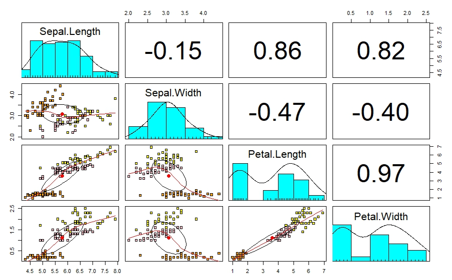
According to this petal length and petal width, sepal length and petal length , Sepal length, and petal width are highly correlated. This leads to multicollinearity. This issue can be reduce using PCA analysis.

#############Principal Component Analysis########################
pca <- prcomp(training[,-5],
             center = TRUE,
             scale. = TRUE)
attributes(pca)

[1] "sdev"     "rotation" "center" 
[4] "scale"    "x"      
$class
[1] "prcomp"
pca$center
Sepal.Length  Sepal.Width Petal.Length
5.8          3.1          3.6
Petal.Width
1.1

pca$scale
Sepal.Length  Sepal.Width Petal.Length
0.82         0.46         1.79
Petal.Width
0.76

print(pca)

Output:
Standard deviations (1, .., p=4):
[1] 1.7173318 0.9403519 0.3843232 0.1371332

Rotation (n x k) = (4 x 4):
                    PC1         PC2        PC3        PC4
Sepal.Length  0.5147163 -0.39817685  0.7242679  0.2279438
Sepal.Width  -0.2926048 -0.91328503 -0.2557463 -0.1220110
Petal.Length  0.5772530 -0.02932037 -0.1755427 -0.7969342
Petal.Width   0.5623421 -0.08065952 -0.6158040  0.5459403

###########summarized#####################
summary(pca)


Output:
Importance of components:
                          PC1    PC2     PC3    PC4
Standard deviation     1.7173 0.9404 0.38432 0.1371
Proportion of Variance 0.7373 0.2211 0.03693 0.0047
Cumulative Proportion  0.7373 0.9584 0.99530 1.0000

######scatter plot## To check the correlation between the principal components ####
  pairs.panels(pca$x,
               gap=0,
               bg = c("orange", "pink", "yellow")[training$Species],
               pch=22)

Output:

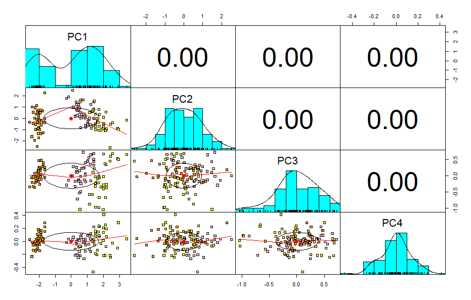
Now there is no correlation between multiple variables therefore there is no  multicollinearity issue.

######### explain the PCA using BY BIPLOT################
library(devtools)
install_github("vqv/ggbiplot")
library(ggbiplot)
g <- ggbiplot(pca,
              obs.scale = 1,
              var.scale = 1,
              groups = training$Species,
              ellipse = TRUE,
              circle = TRUE,
              ellipse.prob = 0.68)
g <- g + scale_color_discrete(name = '')
g <- g + theme(legend.direction = 'horizontal',
               legend.position = 'top')
print(g)

Output:

BIPLOT is useful to understand what is happening in the data set.  

• PC1 is positively correlated with the variables Petal Length, Petal Width, Sepal Length,negatively correlated with Sepal Width.
• PC2 is negatively correlated with Sepal Width.

References

• Principal component analysis (PCA) in R | R-bloggers. (2021, May 7). Principal Component Analysis (PCA) in R | R-bloggers. https://www.r-bloggers.com/2021/05/principal-component-analysis-pca-in-r/